The Transformation of Time and Space

Introduction

\( \def\UP{(\tilde{c}-\tilde{v}){0\rightarrow1}} \def\DO{(\tilde{c}-\tilde{v}){1\rightarrow2}} \def\UPM{|\tilde{c}-\tilde{v}|_{0\rightarrow1}} \def\DOM{|\tilde{c}-\tilde{v}|_{1\rightarrow2}} \def\ds{\displaystyle} \def\mm{ \begin{pmatrix} 1 & 0 & 0 & 0 \\ 0 & 1 & 0 & 0 \\ 0 & 0 & 1 & 0 \\ 0 & 0 & 0 & -1 \end{pmatrix}} \)

In his original article, Einstein elegantly derives the Lorentz transformation of time and space between systems that move at constant velocity relative to each other. Einstein simplified the mathematical derivation by assuming that the relative velocity of the two systems is in the direction of the \(x\) axis, and implicitly assumed (without explicitly discussing it) that the measurement of length, perpendicular to the velocity direction, is the same in both systems. In this section, we will follow the original reasoning of Einstein, and we will

extend the derivation of the Lorentz transformation to the case of a general boost, where a vector of arbitrary direction represents the relative velocity of the two systems
explicitly discuss the conditions on the general form of the Lorentz transformation that preserve the length perpendicular to the velocity.

We will first derive the transformation of time from the synchronization of clocks like Einstein did in his original paper.

Then, using the invariance of the speed of light along with the formalism of bra-ket vectors, we will derive the Lorentz transformation of both time and space in a relatively concise way.

We will assume that the reader is familiar with advanced calculus, linear algebra and the fundamental principles of Special Relativity.

Before getting into the details we define a few concepts and notations that will come in handy as we proceed.

Lorentz Transformation and Events

We consider two systems of reference \(F\) and \(F\) moving at constant velocity \(\vb v\) with respect to each other, where \(\vb v\) is a vector of arbitrary direction. The system \(F\) has spatial coordinates \(x_1\), \(x_2\), \(x_3\) and time \(t\), and \(F’\) has spatial coordinates \(x_1’\), \(x_2’\), \(x_3’\) and time \(t’\).

An observer in \(F\) will identify an event happening at a given place and time by a four-vector \(\vb* X\):

\(\vb* X= (x_1,x_2,x_3,c t)\)

and an observer in \(F’\) will record the same event as \(\vb* X’\):

\({\vb* X’}= (x’_1,x’_2,x’_3,c t’)\)

where \(c\) is the speed of light. We will use sometimes the shorthand version of a four-vector as

\({\vb* X}= ({\vb* x},c t)\)

where \(\vb* x\) is the vector of the spatial coordinates.

The Lorentz transformation describes how the coordinates and the time of the same event observed in \(F\) and \(F’\) are related to each other, and it is assumed to be linear

\begin{equation}
{\vb* X’} = {\bf\Lambda}({\vb* v}) {\vb* X}\label{tran11}
\end{equation}

where \(\vb \Lambda({\vb v})\) is a matrix depending only on the velocity vector \(\vb v\).

bra-ket notation

We introduce now the bra–ket notation for vectors and linear transformations, which will greatly simplify the derivation of the space transformation. The scalar product of two N-dimensional vectors \(\vb{a}\) and \(\vb{b}\) is written in bra-ket notation as

\( \bra{\vb a}\ket{\vb b}\)

In matrix form the bra vector \(\bra{\vb a}\) is represented as a row vector, and the ket vector \(\ket{\vb b}\) is a column vector. A linear transformation in bra-ket form reads

\( \ket{\vb a} \bra{\vb b}\)

which applied to the ket vector \(\ket{\vb c}\) acts as multiplying the vector \(\vb a\) by the scalar product of \(\vb b\) and \(\vb c\)

\begin{align}
\ket{\vb a} \bra{\vb b} \vdot \ket{\vb c} = \ket{\vb a} \bra{\vb b} \ket{\vb c}
\end{align}

The same idea can be used for bra vectors applied to the left of the transformation,

\begin{align}
\bra{\vb c}\vdot \ket{\vb a} \bra{\vb b} = \bra{\vb c}\ket{\vb a} \bra{\vb b}
\end{align}

Transformation of time

In Special Relativity, different observers in the same system of reference looking at the same event will agree that the event has happened at the same time only if their clocks are synchronized. Clocks synchronization is a powerful and central concept in the theory, and it is defined through a thought experiment. We consider two observers in the same system of reference located at different positions A and B. The observer in A sends a photon at time \(t_A\) to the observer in B. The photon arrives in B at \(t_B\), and the observer in B reflects it to A, where it finally comes at time \(t’_A\). The clocks in A and B are synchronized if

\begin{equation}
t_B-t_A = t_A-t_B \label{sync0}
\end{equation}

The synchronization of clocks is the key to get to the transformation of time. Let us now look again at the thought experiment above, but now both from \(F\) and \(F’\),

View from \(F’\)

a photon is emitted at a time \(t’_{0}\) from the origin of \(F’\) along an arbitrary direction
it is reflected at time \(t’_{1}\) by a mirror posed at an arbitrary length from the source
it arrives back at the origin of \(F’\) at time \(t’_{2}\)

Since we assume that the clocks in \(F’\) are synchronized, the following relation holds true:

\begin{equation} \frac{1}{2}(t’_{0}+t’_{2}) = t’_{1} \label{sync} \end{equation}

View from \(F\)

We now look at the three events, emission, reflection and arrival at the source from the perspective of \(F\)

Emission: The photon is emitted from the source at time \(t_{0}\) and at the position

\({\vb v}\, t_{0}\)

where \(\vb v\) is the velocity of \(F’\) measured from \(F\).

Reflection: The photon travels to the mirror with speed \(\vb c_{up}\) and reaches the mirror at a time \(t_{1}\)

\( t_{1} = t_{0} +\ds\frac{ l}{|{\vb c_{up}-\vb v} |} \)

where \(l\) is the distance of the mirror from the source measured from \(F\). When the photon reaches the mirror its position will be

\({\vb v}\, t_{1} + ({\vb c_{up}- \vb v})(t_{1}-t_{0}) = {\vb v}t_{0}+ l\ds\frac{\vb c_{up} }{\|{\vb c_{up}-\vb v} \|}\)

Arrival The time \(t_{2}\) when the photon reaches the source back again is

\(t_{2}= t_{1} +\ds \frac{l}{|{\vb c_{down}-\vb v} |} =t_{0} + \ds\frac{l}{|{\vb c_{up}-\vb v} |}+ \ds\frac{l}{|{\vb c_{down}-\vb v} |}\)

where \(\vb c_{down}\) is the photon velocity on its way back to the source. The position of the photon when it meets the source is,

\({\vb v}t_{2}= {\vb v}t_{0}+{\vb v}\,\space \ds\frac{l}{|{\vb c_{up}-\vb v} |}+ \ds\frac{l}{|{\vb c_{down}-\vb v} |}\)

Considering a general functional relationship \(t’=t'(\vb x,t)\) between the time measured in \(F’\) and in \(F\),

\begin{align*} t’_{0}&=t'({\vb v}\, t_{0} ,t_{0})\\ \\ t’_{1}&=t'({\vb v}t_{0}+ l\ds\frac{\vb c_{up} }{\|{\vb c_{up}-\vb v} \|} , t_{0} + \ds\frac{l}{\|{\vb c_{up}-\vb v} \|} )\\ \\ t’_{2}&=t'( {\vb v}t_{0}+{\vb v}\,\space l(\,\|{\vb c_{up}-\vb v} \|^{-1}+ \,\|{\vb c_{down}-\vb v} \|^{-1}) ,\\ \\ & t_{0} + l(\,\|{\vb c_{up}-\vb v} \|^{-1}+ \,\|{\vb c_{down}-\vb v} \|^{-1}) ) \end{align*}

expanding in Taylor series in \(l\) around the emission event

\begin{align*} t’_{0}&=t'({\vb v}\, t_{0} ,t_{0})\\ t’_{1}&=t'({\vb v}\, t_{0} ,t_{0}) +l \,\,\|{\vb c_{up}-\vb v} \|^{-1} \quad \bra{\grad t’ }\ket{({\vb c_{up}},1)} +o(l^2)\\ t’_{2}&=t'({\vb v}\, t_{0}) + l(\,\|{\vb c_{up}-\vb v} \|^{-1}+ \,\|{\vb c_{down}-\vb v} \|^{-1})\\& \bra{ \grad t’ }\ket{ ({\vb v},1)} +o(l^2) \end{align*}

and using the synchronization condition of Eq.(\ref{sync}), we arrive at the differential equation in \(t’\) (for \(l \to 0\)),

\begin{equation}
\bra{\grad t’}\ket{\vb w}=0
\end{equation}

where,

\begin{align}
{\vb w} =& (\vb v(\,|{\vb c_{up}-\vb v} |^{-1}+ \,|{\vb c_{down}-\vb v} |^{-1}) – 2 {\vb c_{up}}|{\vb c_{up}-\vb v} |^{-1}, \nonumber \ &|{\vb c_{up}-\vb v} |^{-1}- \,|{\vb c_{down}-\vb v} |^{-1}) \nonumber
\end{align}

Assuming a linear relationship between the time in \(F’\) and the coordinates in \(F\)

\(t’ = {\vb p}\cdot \vb x+\beta t\)

where \({\vb p}\) is a vector transforming the spatial coordinates and \(\beta\) is the coefficient transforming time, we arrive at the linear equation in \({\vb p}\) and \(\beta\)

\begin{equation} {\vb p}\vdot [ {\vb v} (\,\|{\vb c_{up}-\vb v} \|^{-1}+ \,\|{\vb c_{down}-\vb v} \|^{-1}) – 2 {\vb c_{up}}\|{\vb c_{up}-\vb v} \|^{-1}] + \beta(\|{\vb c_{up}-\vb v} \|^{-1} – \,\|{\vb c_{down}-\vb v} \|^{-1}) =0 \label{eq2}\end{equation}

Equation (\ref{eq2}) can be further simplified if we look now more in detail to the direction of the vectors \({\vb v}\), \({\vb c_{down}}\) and \({\vb c_{up}}\).

Since the photon in \(F’\) follows the same direction going to the mirror and back to the source, \({\vb c_{down} -\vb v}\) and \({\vb c_{up}-\vb v}\) are parallel, but have different magnitude; hence \({\vb c_{up}}\), \({\vb c_{down}}\) and \({\vb v}\) are all in the same plane, see Fig (1). In the system of reference of three mutually orthogonal unit vectors \({\vb e}_1\), \({\vb e}_2\), and \({\vb e}_3\), with \({\vb e}_1\) and \({\vb e}_2\) in the same plane of \({\vb c{up}}\) and \({\vb v}\), and \({\vb e}_1\) in the same direction of \(\bf v\). the vector \(\bf p\) has components, \( {\vb e}_1 = {\vb v}/{\parallel v\parallel}\), and equation (\ref{eq2}) simplifies to

\begin{equation} \begin{aligned}{\ p_1} { v} (\,|{\vb c_{up}-\vb v} |^{-1}+ \,|{\vb c_{down}-\vb v} |^{-1}) – 2 { c}\,\,(p_1\cos\alpha+p_2\sin\alpha)|{\vb c_{up}-\vb v} |^{-1} \\+\beta\,\,(|{\vb c_{up}-\vb v} |^{-1} – \,|{\vb c_{down}-\vb v} |^{-1}) =0 \end{aligned}\label{eq3}\end{equation}

The component \(p_3\) can be set to zero as it is orthogonal to the plane of \({\vb c_{down}}\) and \({\vb v}\). From

\(\cos\alpha = \ds\frac{\ds c^2 +v^2 – |{\vb c_{up}-\vb v} |^2 }{\ds 2 v c} \)

equation (\ref{eq3}) reads

\begin{equation} p_1 \frac{c^2}{v} +\beta +p_2 \,\,\frac{\ds 2c\sin\alpha |{\vb c_{up}-v} |}{\ds|{\vb c_{up}-v} |-|{\vb c_{down}-v} |} =0\quad\forall \alpha,v \end{equation}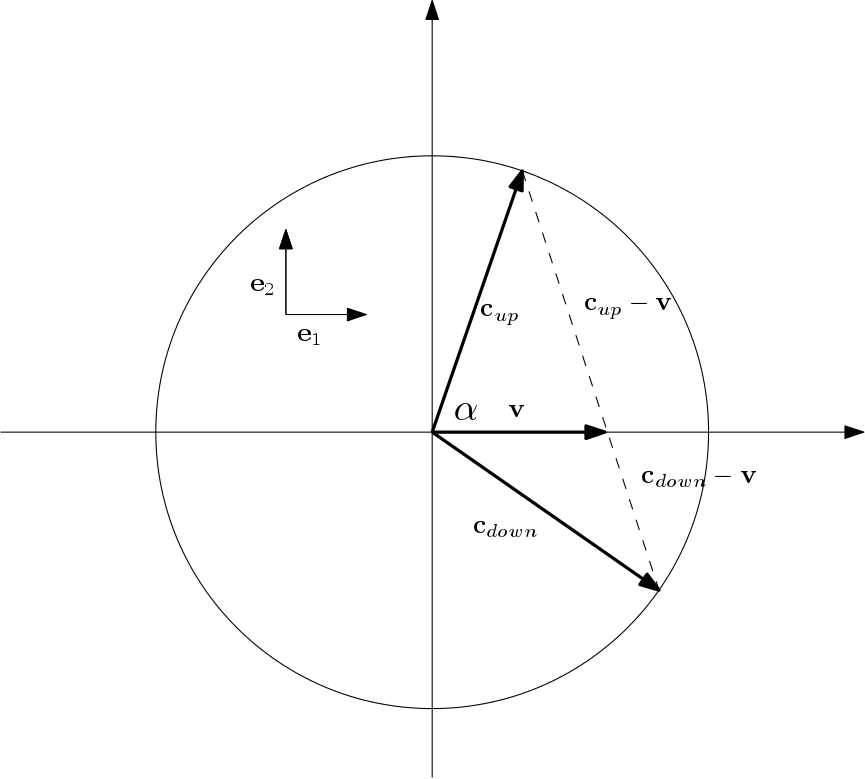

which has solutions

\(p_1=-\beta\frac{v}{c^2}\)

\( p_2=0\)

The transformation of time between \(F’\) and \(F\) becomes then

\begin{equation}
ct’ = \beta\left(-\frac{ v} {c}{\vb e}_1\cdot\vb x+ct \right)\label{timeT}
\end{equation}

where \(\beta\) is a constant depending on the velocity.

Transformation of Space

General Form of the Lorentz Transformation

The Lorentz transformation \(\vb \Lambda({\vb v})\) in its most general form can be represented as a sum of sixteen bra-ket operators formed from a unitary triplet of orthogonal vectors \(\vb e_1\), \(\vb e_2\) and \(\vb e_3\), with \(\vb e_1\) chosen parallel to \(\vb v\)

\begin{equation} \begin{matrix} \lambda_{1,1} \ket{\vb{e}_1,0}\bra{\vb{e}_1,0} & \lambda_{1,2}\ket{\vb{e}_1,0}\bra{\vb{e}_2,0}&\lambda_{1,3}\ket{\vb{e}_1,0}\bra{\vb{e}_3,0}&\lambda_{1,4}\ket{\vb{e}_1,0}\bra{\vb{0},1}\\ % \lambda_{2,1} \ket{\vb{e}_2,0}\bra{\vb{e}_1,0} & \lambda_{2,2}\ket{\vb{e}_2,0}\bra{\vb{e}_2,0}&\lambda_{2,3}\ket{\vb{e}_2,0}\bra{\vb{e}_3,0}&\lambda_{2,4}\ket{\vb{e}_2,0}\bra{\vb{0},1}\\ % \lambda_{3,1} \ket{\vb{e}_3,0}\bra{\vb{e}_1,0} & \lambda_{3,2}\ket{\vb{e}_3,0}\bra{\vb{e}_2,0}& \lambda_{3,3}\ket{\vb{e}_3,0}\bra{\vb{e}_3,0}& \lambda_{3,4}\ket{\vb{e}_3,0}\bra{\vb{0},1}\\ % \lambda_{4,1} \ket{\vb{0},1}\bra{\vb{e}_1,0} & \lambda_{4,2}\ket{\vb{0},1}\bra{\vb{e}_2,0}& \lambda_{4,3}\ket{\vb{0},1}\bra{\vb{e}_3,0}& \lambda_{4,4}\ket{\vb{0},1}\bra{\vb{0},1}\\ \end{matrix} \label{generalLambda} \end{equation}

The synchronization of clocks and the invariance of the space-time interval are used to determine the transformation but are not sufficient to identify all sixteen free parameters: assumptions need to be made on how events are observed in \(F\) and \(F’\) to restrict the possible choices for \(\Lambda(\vb v)\).

The time component of an event in \(F\) will only affect the spatial component in \(F’\) along the velocity direction \(\ket{\vb e_1}\),

\begin{equation}
\vb \Lambda({\vb v} (x_4 \ket{ \vb{ 0},1} )=x_4(\lambda_{1,4}\ket{\vb{ e}_1,0}+\lambda_{2,4}\ket{\vb{ e}_2,0} +\lambda_{3,4}\ket{\vb{ e}_3,0} +\lambda_{4,4}\ket{ \vb{ 0},1})
\end{equation}

which is \(\lambda_{2,4}=\lambda_{3,4}=0\).

The direction \(\vb e_1\) is invariant. Hence, for an event in \(F\),

\begin{equation}
\vb \Lambda({\vb v}) ( x_1\ket{\vb{ e}_1,0} + x_4 \ket{ \vb{ 0},1}) = x_1\,(\lambda_{1,1}\ket{\vb{ e}_1,0}+\lambda_{2,1}\ket{\vb{ e}_2,0} +\lambda_{3,1}\ket{\vb{ e}_3,0} +\lambda_{4,1}\ket{ \vb{ 0},1}) +x_4(\lambda_{1,4}\ket{\vb{ e}_1,0} +\lambda_{4,4}\ket{ \vb{ 0},1})
\end{equation}

\(\lambda_{2,1}=\lambda_{3,1}=0\). Equation \(\ref{generalLambda}\) simplifies thus as,

\begin{equation} \begin{matrix} \lambda_{1,1} \ket{\vb{e}_1,0}\bra{\vb{e}_1,0} & \lambda_{1,2}\ket{\vb{e}_1,0}\bra{\vb{e}_2,0}&\lambda_{1,3}\ket{\vb{e}_1,0}\bra{\vb{e}_3,0}&\lambda_{1,4}\ket{\vb{e}_1,0}\bra{\vb{0},1}\\ % & \lambda_{2,2}\ket{\vb{e}_2,0}\bra{\vb{e}_2,0}&\lambda_{2,3}\ket{\vb{e}_2,0}\bra{\vb{e}_3,0}&\\ % & \lambda_{3,2}\ket{\vb{e}_3,0}\bra{\vb{e}_2,0}& \lambda_{3,3}\ket{\vb{e}_3,0}\bra{\vb{e}_3,0}& \\ % \lambda_{4,1} \ket{\vb{0},1}\bra{\vb{e}_1,0} & \lambda_{4,2}\ket{\vb{0},1}\bra{\vb{e}_2,0}& \lambda_{4,3}\ket{\vb{0},1}\bra{\vb{e}_3,0}& \lambda_{4,4}\ket{\vb{0},1}\bra{\vb{0},1}\\ \end{matrix} \label{generalLambda_1} \end{equation}

The spatial component along \(\ket{\vb{ e}_2,0}\) and \(\ket{\vb{ e}_3,0}\) of any event preserve their direction and length under \(\vb \Lambda({\vb v})\).

\begin{equation}
\vb \Lambda({\vb v}) \, (x_2\ket{ \vb{ e}_2,0}+x_3\ket{ \vb{ e}_3,0}) = x_2\,(\lambda_{1,2}\ket{\vb{ e}_1,0}+\lambda_{2,2}\ket{\vb{ e}_2,0} +\lambda_{3,2}\ket{\vb{ e}_3,0}) + x_3\,(\lambda_{1,3}\ket{\vb{ e}_1,0}+\lambda_{2,3}\ket{\vb{ e}_2,0} +\lambda_{3,3}\ket{\vb{ e}_3,0})
\end{equation}

condition equivalent to \(\lambda_{1,2}=\lambda_{1,3}=\lambda_{2,3}=\lambda_{3,2}=0\) and \(\lambda_{2,2}=\lambda_{3,3}=1\).

Using the conditions above, \(\vb \Lambda({\vb v})\) simplifies further as

\begin{equation} \begin{matrix} \lambda_{1,1} \ket{\vb{e}_1,0}\bra{\vb{e}_1,0} & &&\lambda_{1,4}\ket{\vb{e}_1,0}\bra{\vb{0},1}\\ % & \ket{\vb{e}_2,0}\bra{\vb{e}_2,0}&\\ % && \ket{\vb{e}_3,0}\bra{\vb{e}_3,0}& \\ % \lambda_{4,1} \ket{\vb{0},1}\bra{\vb{e}_1,0} & \lambda_{4,2}\ket{\vb{0},1}\bra{\vb{e}_2,0}& \lambda_{4,3}\ket{\vb{0},1}\bra{\vb{e}_3,0}& \lambda_{4,4}\ket{\vb{0},1}\bra{\vb{0},1}\\ \end{matrix} \label{generalLambda_2} \end{equation}

and with equation (\ref{timeT}), we arrive at the final functional form of \(\vb \Lambda({\vb v})\)

\begin{equation} \vb \Lambda({\vb v})= \lambda_{1,1} \ket{\vb{e}_1,0}\bra{\vb{e}_1,0} + \lambda_{1,4}\ket{\vb{e}_1,0}\bra{\vb{0},1}+ \ket{\vb{e}_2,0}\bra{\vb{e}_2,0}+ \ket{\vb{e}_3,0}\bra{\vb{e}_3,0} -\beta\frac{ v} {c} \ket{\vb{0},1}\bra{\vb{e}_1,0} +\beta \ket{\vb{0},1}\bra{\vb{0},1}\\ \label{simpleLambda_v1} \end{equation}

The constants \(\lambda_{1,1}, \lambda_{2,2}, \lambda_{3,3},\) and \(\beta\) must be positive to prevent axis reflection.

Invariance of Light Speed

In Special Relativity the spacetime interval between two events \((x_1,y_1,z_1,ct_1)\) and \((x_2,y_2,z_2,ct_2)\) is defined as

\begin{equation}\Delta s^2 = (x_2-x_1)^2 + (y_2-y_1)^2 + (z_2-z_1)^2 -c^2 (t_2-t_1)^2 \end{equation}

and can be written in bi-linear form as

\begin{align*}\Delta s^2 &= \bra{\vb* X}\ket{ \vb M \vb* X} \\ \vb* X&= (x_2-x_1,y_2-y_1,z_2-z_1,c (t_2-t_1))
\end{align*}

where

\begin{equation}
{\vb M}=\mm
\end{equation}

A spacetime interval measured in \(F’\) is linked to the same interval in \(F\) by the Lorentz transformation

\begin{align*} \Delta s’^2 &= \bra{\vb* X’}\ket{ \vb M \vb* X’}= \bra{{\vb \Lambda}\vb*{X}}\ket{ {\vb M} {\vb \Lambda}\vb*{X}}\\ &=\bra{\vb*{X}}\ket{ {\vb \Lambda}^T{\vb M} {\vb \Lambda}\vb*{X}} \end{align*}

In the system \(F\) we consider a photon moving along an unitary vector \(\vb n\). The photon at time \(t_1\) is in the position \(\vb x_1\), and moves to the position \(\vb x_1+{\vb n}\,c(t_2-t_1)\) at the time \(t_2\). The spacetime interval in \(F\) of the two events is identically zero,

\begin{equation*}\Delta s^2 = \Vert{\vb n}\Vert c^2(t_2-t_1)^2-c^2(t_2-t_1)^2 \end{equation*}

As we are considering two events along the path of a photon (the so-called world line of a photon), the spacetime interval \(\Delta’ s^2\) in \(F’\) must also be zero,

\begin{equation} \bra{({\vb n}\,c(t_2-t_1),c(t_2-t_1))}\ket{ {\vb \Lambda}^T{\vb M} {\vb \Lambda}\cdot({\vb n}\,c(t_2-t_1),c(t_2-t_1))}=0\end{equation}

equivalent to,

\begin{equation}\bra{({\vb n},1)}\ket{ {\vb \Lambda}^T{\vb M} {\vb \Lambda}\cdot({\vb n} ,1)}=0 \label{rt1l}\end{equation}

for all \(\vb n\) such that \(||\vb n||=1\).

To solve equation (\ref{rt1l}) we need \({\vb M} {\vb \Lambda}\), which is \({\vb \Lambda}\) with the time component changed sign,

\begin{equation} {\vb M} \vb \Lambda({\vb v})= \lambda_{1,1} \ket{\vb{e}_1,0}\bra{\vb{e}_1,0} + \lambda_{1,4}\ket{\vb{e}_1,0}\bra{\vb{0},1}+ \lambda_{2,2}\ket{\vb{e}_2,0}\bra{\vb{e}_2,0}+ \lambda_{3,3}\ket{\vb{e}_3,0}\bra{\vb{e}_3,0} +\beta\frac{ v} {c} \ket{\vb{0},1}\bra{\vb{e}_1,0} -\beta \ket{\vb{0},1}\bra{\vb{0},1} \label{simpleLambda_v11} \end{equation}

and \( {\vb \Lambda}^T\) is readily obtained by exchanging the bra and ket vectors,

\begin{equation} \vb \Lambda({\vb v})^T= \lambda_{1,1} \ket{\vb{e}_1,0}\bra{\vb{e}_1,0} + \lambda_{1,4}\ket{\vb{0},1}\bra{\vb{e}_1,0}+ \lambda_{2,2}\ket{\vb{e}_2,0}\bra{\vb{e}_2,0}+ \lambda_{3,3}\ket{\vb{e}_3,0}\bra{\vb{e}_3,0} -\beta\frac{ v} {c} \ket{\vb{e}_1,0}\bra{\vb{0},1} +\beta \ket{\vb{0},1}\bra{\vb{0},1} \label{simpleLambda_v12} \end{equation}

The product \(\vb \Lambda({\vb v})^T{\vb M} \vb \Lambda({\vb v})\) is

\begin{equation} \begin{matrix} (\lambda_{1,1}^2-\beta^2\frac{v^2} {c^2}) \ket{\vb{e}_1,0}\bra{\vb{e}_1,0} + (\lambda_{1,1}\lambda_{1,4}+\beta^2\frac{v} {c})\ket{\vb{0},1}\bra{\vb{e}_1,0} + (\lambda_{1,1}\lambda_{1,4}+\beta^2\frac{v} {c})\ket{\vb{e}_1,0}\bra{\vb{0},1}+\\ \lambda_{2,2}^2\ket{\vb{e}_2,0}\bra{\vb{e}_2,0}+ \lambda_{3,3}^2\ket{\vb{e}_3,0}\bra{\vb{e}_3,0} +(\lambda_{1,4}^2-\beta^2) \ket{\vb{0},1}\bra{\vb{0},1} \end{matrix} \label{simpleLambda_v13} \end{equation}

and equation \(\ref{rt1l}\) reads,

\begin{equation} (\lambda_{1,1}^2-\beta^2\frac{v^2} {c^2}) n_1^2 + 2(\lambda_{1,1}\lambda_{1,4}+\beta^2\frac{v} {c})n_1 + n_2^2 + n_3^2 +(\lambda_{1,4}^2-\beta^2) =0 \label{simpleLambda_v13l} \end{equation}

Choosing \(n_2\) or \(n_3=1\) and \(n_1=0\),

\begin{equation} (\lambda_{1,4}^2-\beta^2) =-1 \end{equation}

Choosing \(n_1=\pm 1\) and \(n_2=n_3=0\),

\begin{gather} (\lambda_{1,1}^2-\beta^2\frac{v^2} {c^2}) + 2(\lambda_{1,1}\lambda_{1,4}+\beta^2\frac{v} {c}) +(\lambda_{1,4}^2-\beta^2) =0 \\ (\lambda_{1,1}^2-\beta^2\frac{v^2} {c^2}) – 2(\lambda_{1,1}\lambda_{1,4}+\beta^2\frac{v} {c}) +(\lambda_{1,4}^2-\beta^2) =0 \end{gather}

and we arrive at the system of equations

\begin{equation} \begin{matrix} \lambda_{1,1}^2-\ds\beta^2\frac{v^2} {c^2} &= 1 \\ \lambda_{1,1}\lambda_{1,4}+\ds\beta^2\frac{v} {c} & =0 \\ \lambda_{1,4}^2-\beta^2 &=-1 \\ \end{matrix} \end{equation}

which has the only admissible solutions,

\begin{align*} \beta&=\ds\frac{1}{\ds\sqrt{1-\frac{v^2}{c^2} }}\\ \lambda_{1,1}&= \beta \\ \lambda_{1,4}&=-\ds\frac{v}{c}\beta \\ \end{align*}

The Lorentz transformation takes the final form

\begin{equation} \vb \Lambda({\vb v})= \beta \ket{\vb{e}_1,0}\bra{\vb{e}_1,0} -\ds\beta\frac{v}{c}\ket{\vb{e}_1,0}\bra{\vb{0},1}+ (\vb{I’}-\ket{\vb{e}_1,0}\bra{\vb{e}_1,0}) -\beta\frac{ v} {c} \ket{\vb{0},1}\bra{\vb{e}_1,0} +\beta \ket{\vb{0},1}\bra{\vb{0},1}\\ \label{lambda_1} \end{equation}

where the operator \(\vb I’\) is the identity for the components \(\ket{\vb{e}_1,0}, \ket{\vb{e}_2,0}\) and \(\ket{\vb{e}_3,0}\) ,

\begin{equation} \ket{\vb{e}_2,0}\bra{\vb{e}_2,0}+ \ket{\vb{e}_3,0}\bra{\vb{e}_3,0} = {\vb{I’}}-\ket{\vb{e}_1,0}\bra{\vb{e}_1,0} \end{equation}

The inverse of \(\Lambda(v)\) transforms the coordinates from \( F’\) to \(F\) and can be readily obtained by exchanging the velocity sign,

\begin{equation} \underbrace{\begin{matrix} \beta \ket{\vb{e}_1,0}\bra{\vb{e}_1,0} & &&-\ds\frac{v}{c}\beta \ket{\vb{e}_1,0}\bra{\vb{0},1}\\ % & \ket{\vb{e}_2,0}\bra{\vb{e}_2,0}&\\ % && \ket{\vb{e}_3,0}\bra{\vb{e}_3,0}& \\ % -\beta\ds\frac{v}{c} \ket{\vb{0},1}\bra{\vb{e}_1,0} & & & \beta\ket{\vb{0},1}\bra{\vb{0},1}\\ \end{matrix}}_{\Lambda(\vb{v})} \times \underbrace{\begin{matrix} \beta \ket{\vb{e}_1,0}\bra{\vb{e}_1,0} & &&\ds\frac{v}{c}\beta \ket{\vb{e}_1,0}\bra{\vb{0},1}\\ % & \ket{\vb{e}_2,0}\bra{\vb{e}_2,0}&\\ % && \ket{\vb{e}_3,0}\bra{\vb{e}_3,0}& \\ % \beta\ds\frac{v}{c} \ket{\vb{0},1}\bra{\vb{e}_1,0} & & & \beta\ket{\vb{0},1}\bra{\vb{0},1}\\ \end{matrix}}_{\Lambda^{-1}=\Lambda(-\vb{v})} = {\vb{I}} \label{generalLambda_r2} \end{equation}

The Lorentz transformation written explicitly in terms of the velocity vector, as \( \ket{\vb{e}_1,0}=\ket{\vb{v},0}/v\), reads,

\begin{equation} \vb \Lambda({\vb v})= \frac{\beta}{v^2} \ket{\vb v,0}\bra{\vb{v},0} -\ds\frac{\beta}{c}\ket{\vb{v},0}\bra{\vb{0},1}+ (\vb{I’}-\frac{1}{v^2}\ket{\vb{v},0}\bra{\vb{v},0}) -\frac{ \beta} {c} \ket{\vb{0},1}\bra{\vb{v},0} +\beta \ket{\vb{0},1}\bra{\vb{0},1}\\ \label{lambda_123} \end{equation}

The derivation of the relativistic Maxwell equations will be easier when the time component \(t\) in the Lorentz transformation is in time units, not space \(ct\),

\begin{equation} \vb \Lambda'({\vb v})= \frac{\beta}{v^2} \ket{\vb v,0}\bra{\vb v,0} -\ds\beta\ket{\vb v,0}\bra{\vb{0},1}+ (\vb{I’}-\frac{1}{v^2}\ket{\vb{v},0}\bra{\vb{v},0}) -\frac{ \beta} {c^2} \ket{\vb{0},1}\bra{\vb v,0} +\beta \ket{\vb{0},1}\bra{\vb{0},1}\\ \label{lambda_11} \end{equation}

Finally, when \(\vb v\) has the direction of the x-axis, the transformation simplifies to the original Einstein formula

\begin{align} x’ &= \beta(x-vt ) \nonumber\\ y’&=y\nonumber\\ z’&=z\nonumber\\ t’&= \beta\left(t-\ds\frac{v}{c^2}x \right)\label{Lorentz} \end{align}

Finally, from equation (\(\ref{simpleLambda_v13l}\)), the Lorentz transformation satisfies the condition \({\vb \Lambda}^T{\vb M} {\vb \Lambda}=\vb M\), hence \(\Delta’ s=\Delta s\) for all events, not only those on a world line of a photon,

\begin{equation} \Delta s’^2 = \bra{\vb* X’}\ket{ \vb M \vb* X’}= \bra{{\vb \Lambda}\vb*{X}}\ket{ {\vb M} {\vb \Lambda}\vb*{X}}=\bra{\vb*{X}}\ket{ {\vb \Lambda}^T{\vb M} {\vb \Lambda}\vb*{X}}=\bra{\vb*{X}}\ket{ {\vb M} \vb*{X}}=\Delta s\label{nrm} \end{equation}